EXTENDED ESSAY IN BIOLOGY
INTERTIDAL ZONATION OF HALOSACCION GLANDIFORME:
A FOCUS ON HEIGHT AND SLOPE AS FACTORS OF ZONATION
LESTER B. PEARSON COLLEGE
ALEX C. FLETCHER
JANUARY 14, 2002
ABSTRACT:
An intertidal study of the organism Halosaccion glandiforme was performed at Race Rocks Marine Protected Area a unique and undisturbed island located seventeen kilometres southwest of Victoria in the Strait of Juan de Fuca . Belt transects from three similar locations on the island were taken from the zero tide level up past the high tide mark. These transect photos were combined with other measurements and calculations to look at the variables influencing growth in the intertidal zone. The intertidal zone is unique in its numerous abiotic and biotic factors that influence life in the region. For the purpose of this study two of these factors were chosen in an attempt to quantify the possible relation that exists between them and the ecological niche of Halosaccion glandiforme. Vertical elevation from the zero tide level and angle of inclination of the rocky shore were compared with population density of the species. While analysis of slope and population density relation proved fairly inconclusive, simple statistical testing showed that a trend does exist between intertidal height and population density of Halosaccion glandiforme.
Table of Contents
List of Figures and Tables
Introduction…………………………………………………………………………1
The Problem
Purpose and Background of the Study
Hypotheses
Limitations
Review of Literature and Related Research…………………………..……….3
Introduction, Information about the organism
The Theory
Research Results in Related Areas
Research Design and Procedures………………………………………………7
The Setting and Population of the Study
The Experimental and Control Groups Used
Instruments Used
Analysis of Data……………………………………………………………….…10
Introduction
Findings that Relate to Hypotheses 1 and 2
Statistical Analysis
Findings that Relate Hypotheses 3 and 4
Conclusions and Recommendations for Further Study…………….…….20
Interpretations and Implications of the Findings
Recommendations
References Cited…………………………………………………………..…..…22
Appendix…………………………………………………………………………..23
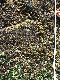
Transect-peg 5
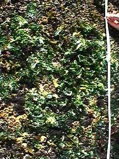
Transect-peg 5b1
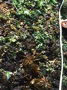
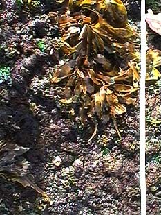
Transect-peg 6
List of Figures and Tables
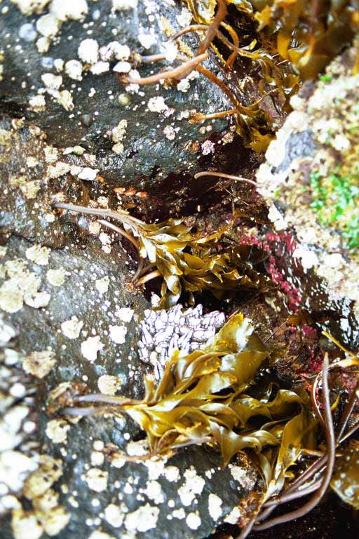
Figure 1. A small cluster of Halosaccion glandiforme, among barnacles, is shown growing next to a tide pool. …………………………………………………………………………. 1
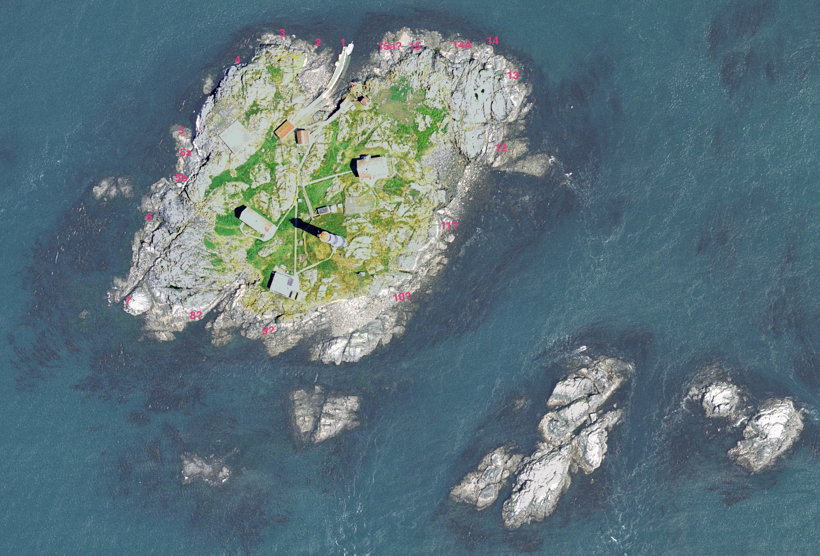
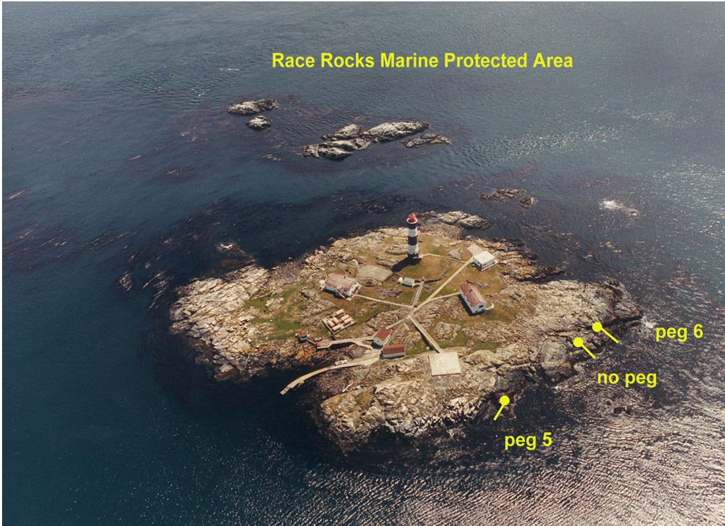
Figure 3. Areal view of Race Rocks Marine protected Area. Yellow markers indicate locations of study pegs and belt transect line ……………………………………………… 6
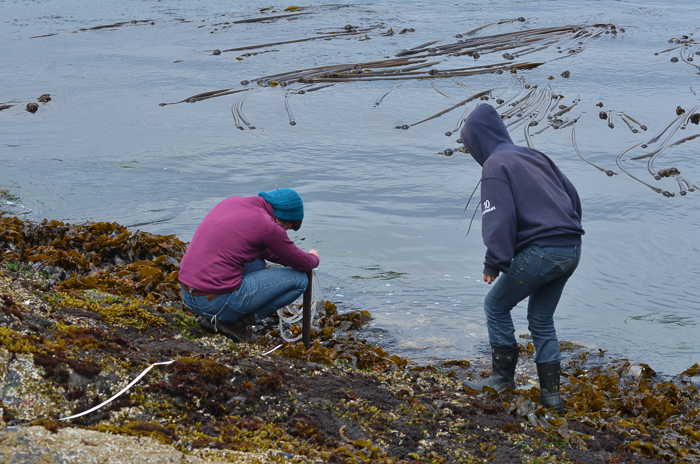
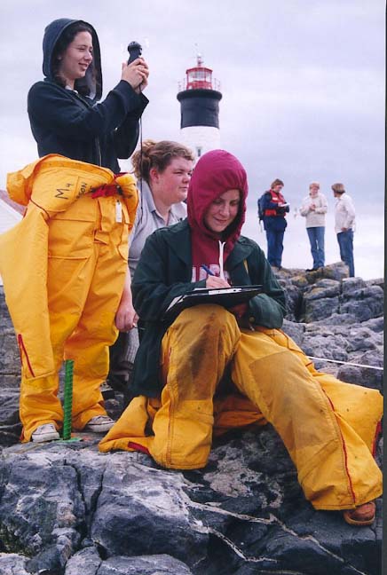
Figure 4. Working with H.glandiforme at the race Rocks Marine Protected Area…………………………………………………………………………………………………………7
Figure 5. This image represents an example of a meter segment from the belt transect (taken from peg 6 at meter 4). …………………………………………………………………….. 8
Figure 6. This image is an example of a meter segment from a belt transect (peg6, meter segment 4). ………………………………………………………………………………………. 9
Table 1. Population density (in percent coverage of each meter segment) is shown in relation to the mean
of vertical height of the corresponding meter segment from measurements at peg 5. ………………………………………………………………………………………………………….. 10
Table 2. Population density (in percent coverage of each meter segment) is listed in relation to the mean of vertical height of the corresponding meter segment from measurements at peg 5b1. …………………………………………………………………. 10
Table 3. Population density (in percent coverage from each meter segment) is shown in relation to the mean of vertical height of the corresponding meter segment from measurements at peg 6. ……………………………………………………………………… 10
Figure 7. Graph of data from table one, peg 5.………………………………………… 11
Figure 8. Graph of data from table 2, peg 5b1.………………………………………… 11
Figure 9. Graph of data from table 3, peg 6……………………………………………… 12
Figure 10. Graph of population density in relation to mean of intertidal vertical height with
the three belt transects combined. ………………………………………………………….. 12
Table 4. Table of combined data of the significant values for the analysis of normal distribution from three pegs. …………………………………………………………………… 13
Table 5. Data table of expected normal distribution values and obtained distribution values used in conjunction to perform chi-squared test.………………………………………… 13
Figure 11. Graph of percent coverage vs. vertical height, comparing obtained values to normal distribution values………………………………………………………………………… 14
Figure 12. Graph of peg 5, belt transect terrain profile. ………………………………. 15
Figure 13. Graph of peg 5b1, belt transect terrain profile…………………………….. 16
Figure 14. Graph of peg 6, belt transect terrain profile………………………………… 17
Table 6. This data shows percent coverage in relation to the slope of the intertidal zone. ………………………………………………………………………………………………………….. 18
Figure 15. Graph of table 6, the relation between population density and intertidal slope……………………………………………………………………………………………………..18
Introduction
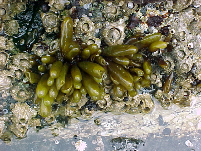
Figure 1. A small cluster of Halosaccion glandiforme among barnacles, ius shown growing next to a tidepool
The Problem:The purpose of this study is to try and quantify certain factors that are a part of the ecological niche of the sea sac Halosaccion glandiforme (figure 1) from the Rhodophyta division. From observing this plant on numerous occasions it is clear that this organism grows in a limited vertical range on the intertidal zone, the threshold between marine aquatic and terrestrial environments. It is likely that a specific physical setting exists for this species, and similarly with other intertidal species, where growing conditions are optimal. The main focus will be to look at the extent to which slope and elevation, in the tidal zone, affect the ideal habitat conditions of the Halosaccion glandiforme.
Purpose and background of the Study
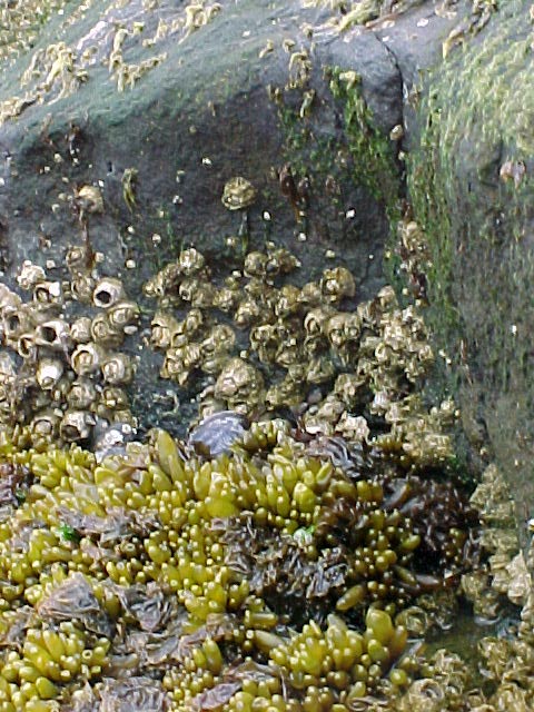
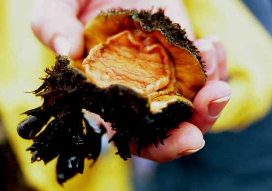
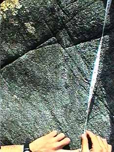
Figure 2. Picture showing Halosaccion glandiforme growing up to but not on a vertical surface.
Similar to all rocky intertidal dwelling species Halosaccion glandiforme is well adapted to survive the dynamic conditions presented in this ecosystem. This zone is characterized by the rapid changes and variability of temperature, light, moisture, salinity, and water movement. The aqua dynamics of the sea sac’s streamlined shape decreases the friction between it and the constantly moving marine waters. H. glandiforme are well anchored to surfaces (usually rock) by strong attachment devices as well as by growing in clusters of its own kind it is more protected. Being a water-filled sac the plant is less susceptible to the changes in moisture and temperature as a result of the tidal waters that are more limiting to other algae such as sea lettuce (Ulva fenestrata) and Purple laver (Porphyra perforata). From observations a growth trend along certain elevations, where the appropriate conditions of moisture and sunlight are found, appears to exist for H. glandiforme and other intertidal species. Also based on observation (figure 2) it seems as though the inclination of rock
surface influences the location of intertidal species including the H. glandiforme. This may be caused by the force of water movement along flatter, less restrictive surfaces, compared to steeper surfaces where friction between rock and water results in turbulence and a rough growing site for organisms. The characteristics and adaptations of each intertidal organism determine its niche. In looking at some of the many determining variables that exist along the seashore we can attempt to quantify this area.
Hypotheses
Hypothetically there is a measurable height at which this alga prospers as well as a preferred degree of inclination for its growth. A higher density population trend along the intertidal zone at this level would represent this.
- Ho- There is no significant relation between Halosaccion glandiforme population density and the vertical elevation on the tidal zone.
- Ha- there is a significant relation between Halosaccion glandiforme population density and the vertical elevation on the tidal zone
- Ho- There is no significant relation between inter tidal angle of slope and population density of the Halosaccion glandiforme.
- Ha- There is a significant relation between inter tidal angle of slope and population density of the Halosaccion glandiforme.
Limitations
This study is limited by only taking data at one point in the growing season of the plant and by not having the time to repeat collections of data several times over an extended period of time. The site of study, performed at Race Rocks Marine Protected Area is a prime location for flourishing intertidal life. However, taking measurements and data from three locations in one confined area is limiting in respect to the broadness of the viability of the results. Due to restrictions of time it was not possible to explore further relations and effects of abiotic and biotic factors. In addition many of the highly influential factors (such as wave motion, temperature, etc.) are not easily quantified and are not easily controlled thereby limiting the accuracy and broadness of the study and it’s findings.
Review of Literature and Related Research
Introduction, Information about the Organism
Specific information on Halosaccion glandiforme is limited beyond short physical descriptions and categorization. In Pacific Coastal marine texts Halosaccion is often referred to for its intertidal qualities while actual studies on the plant were not found while researching the topic. Typical descriptions of Halosaccion glandiforme depict the plant as a thin-walled elongated sausage-shaped sac found in the mid-intertidal region of rock dominated shores. The plant is identifiable by its rounded head and short stipe anchored by a small circular holdfast. Also, resulting from the water it contains, applying pressure to the plant produces fine sprays of water emitted from the pores. In Common Seaweeds of the Pacific Coast (by J. Robert Waaland) it is stated that “Halosaccion glandiforme may reach lengths up to 25 cm and 3 to 4 cm in diameter; typical sizes are about 15 cm long by 2 to 3 cm in diameter.” The maximum length (25cm) is far greater than those studied in this paper. Typical sizes, in the populations and the physical vicinity of the study for this paper, were closer to a range of 1 to 10 cm in length.
The Theory
While theory in the area of inter tidal zone life is limited there is literature that states observations relating to the structured zonation that occurs in the intertidal zone. The slope hypothesis is related to a general description of the influence of shoreline gradient on intertidal zonation provided in Pacific Seashores A Guide to Intertidal Ecology (Carefoot, 1977). “Generally, where the range of the tides is small, or where the slope of the beach is steep, the bands are narrow; where the range of the tides is great, or where the slope of the beach is flat, the zones are wide.” From this statement it is clear that physical factors such as slope are influential on the intertidal zonation and banding of species. In Seashore Life of the Northern Pacific (Kozloff, 1996) it is stated that “On flat-topped reefs and rocks that do not have steep slopes, there should be plenty of Halosaccion glandiforme.” This provides a basis for the concept that shoreline gradient is plausible as a factor influencing the growth of Halosaccion. Therefore such factors of the intertidal zone directly affect the band of ideal growing conditions for organisms.
A theoretical description for universal zonation is presented by Stephenson’s “universal” scheme of zonation (Stephenson, 1949). This scheme is representative of the diverse zonal patterns around the world. It divides tidal shores into five main categories. From highest to lowest is the Supralittoral zone above the tidemark being mainly terrestrial however influenced by spray from waves and ocean mist. Below is the supralittorial fringe that encompasses the upper intertidal zone including the highest living barnacle and lowest limits of lichens. The Midlittoral zone is the whole intertidal area from the most elevated barnacles to the most elevated brown algae. The lowest edge of the intertidal zone represents the beginning of the Infralittoral fringe that continues to the lowest mark visible between waves at low tide. Bellow is the final tidal zone called the Infralittoral zone being almost constantly submerged. In this scheme Halosaccion glandiforme is situated between the extreme high water mark and the extreme low water mark somewhat centrally in the midlittoral zone.
Research Results in related areas
The most significant research results that relate to this paper involve work done on the abiotic features that affect the growth of intertidal organisms. While the research is not specific to Halosaccion glandiforme it is relevant to the intertidal zone occupied by this species.
The primary factor in determining growing location for algae results from the production of their many spores and the conditions that affect where the spores choose to settle. The few spores that survive and continue to develop into their gametophyte forms will only survive if they are in appropriate niche for that species.
There is much research that has gone into the effect of tidal levels and variation on zonation. The theory of zonation is based on the relationship between intertidal zones and tide levels. However it is not “universal” as it has been found (even by the Stephensons) to be inaccurate in certain situations. This comes from the influence of other factors that cause variance between intertidal zones and that must be considered when studying this area. The cycles that tides go through, in accordance with the sun and predominantly the moon, will affect the intertidal zone configuration by controlling the submersion of the intertidal zone and its organisms.
The upper limits of the intertidal zone are subject to temperature fluctuations and other abiotic terrestrial environmental factors such as air movement and fresh water that effect growth. Water retention enables certain species to survive for longer periods of time out of the water and therefore higher in the intertidal zone. The effects of exposure on seaweeds has been studied by Kanwisher (Kanwisher, J, 1957). In his article “Freezing and drying in intertidal algae” he measures water loss in certain algal species of the intertidal area. A brown alga Fucus vesiculosus was recorded as having lost 91% of its moisture to evaporation from solar heat. In laboratory work performed he found that this level of evaporation would occur in a period of about an hour and half. Similarly Enteromorpha linza demonstrated an 84 percent loss of water and Ulva lactuca a 77 percent loss of water when subject to terrestrial conditions. It is likely that the structure of Halosaccion glandiforme, being a water retentive sac, permits for lengthier exposure time with a higher level of water retention.
Light is a very influential aspect on intertidal life and zonation. As the source for photosynthesis it is vital to plant life. However it is also harmful in that ultra violet light can damage plant tissue. The sun’s UV rays can bleach marine plants that spend extended periods of time out of the water.
There is also the factor of competition for growing space amongst the many species and individuals occupying the limited space of the intertidal zone. As well predation and grazing by herbivores will affect the growing conditions of intertidal species. The abrasive action by waves is a determinate in zonation separating stronger better-adapted organisms from those that are not able to endure the conditions. Some organisms have greater survivability in such conditions through growing in clusters, having streamlined shapes, sturdy holdfasts, and other such features.
Research Design and Procedures

Figure 3, Aerial view of Race Rocks Ecological Reserve. Yellow markers denote location of study pegs and belt transect lines.
The Setting and Population of the Study
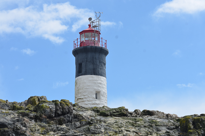
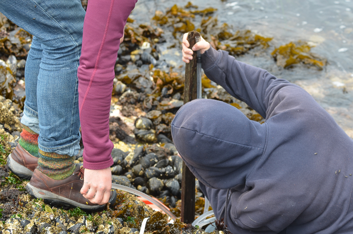
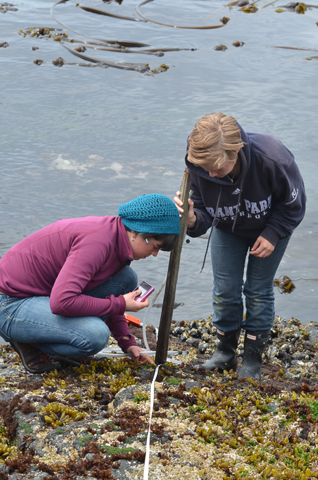
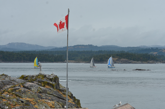
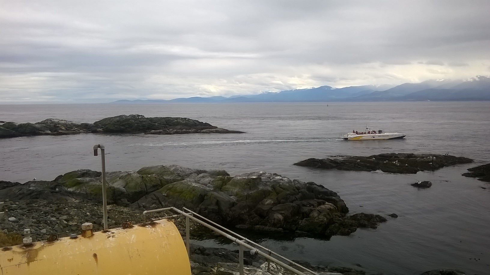
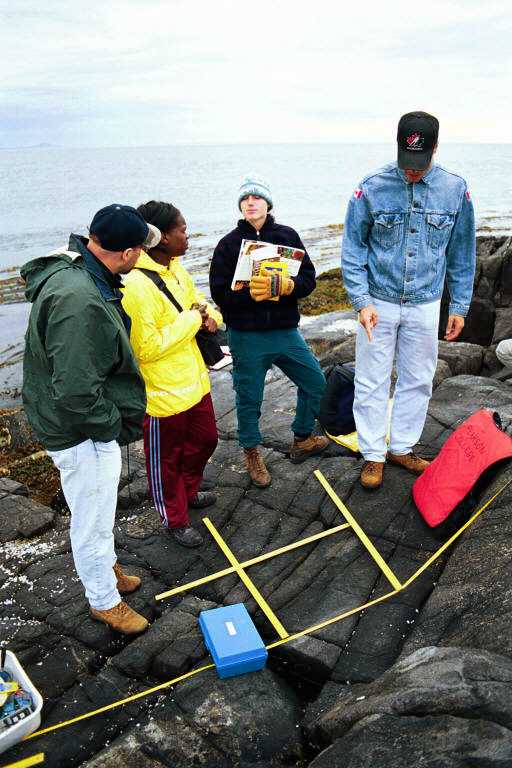
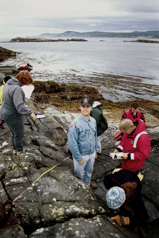
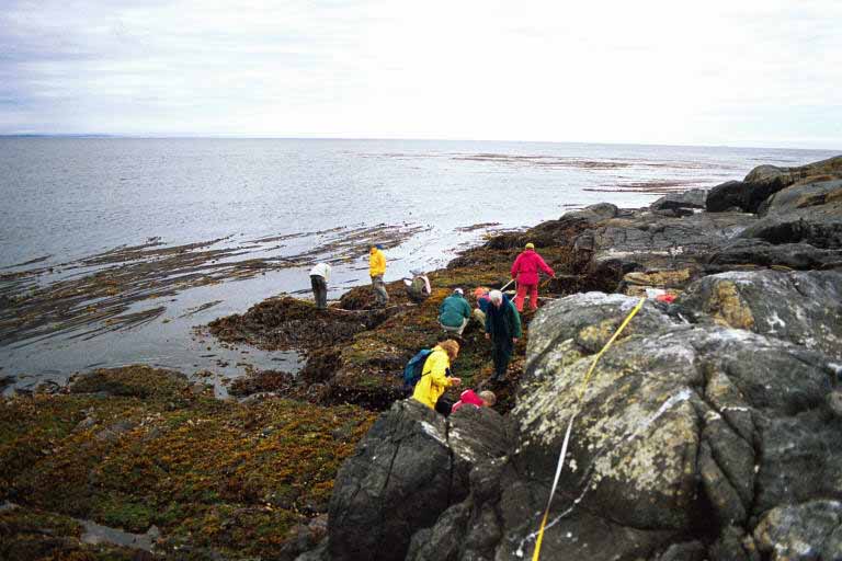
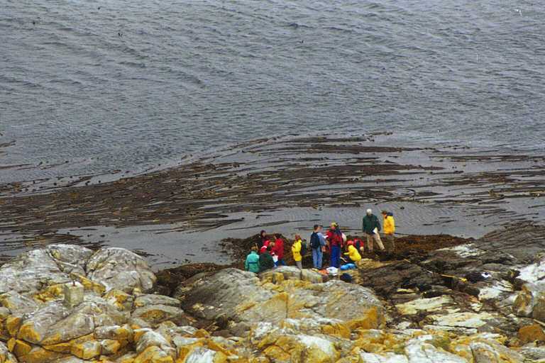
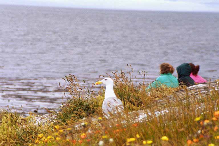
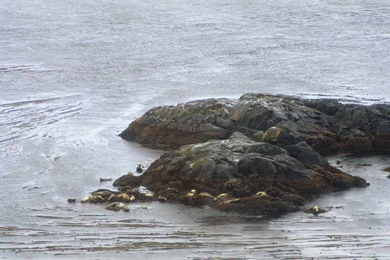
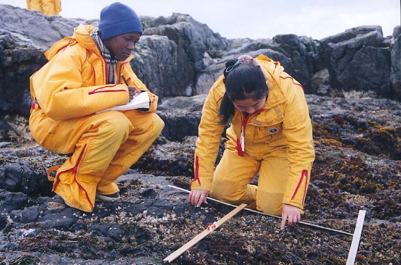
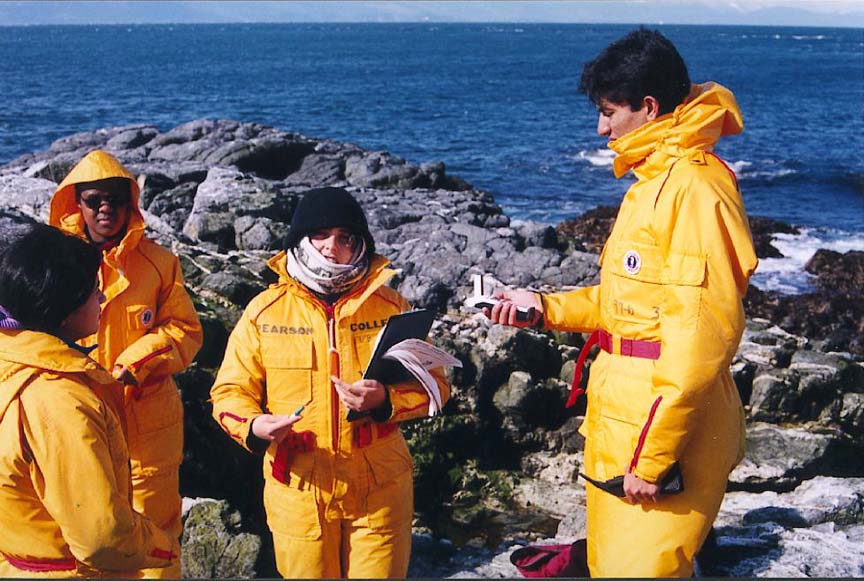
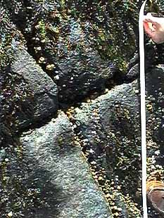
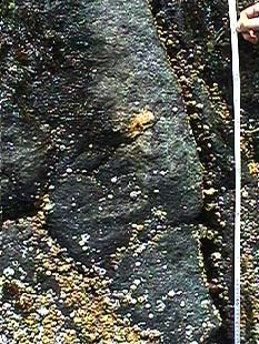
The data collection for this study was carried out at Race Rocks Marine Protected Area located 17 kilometres southwest of Victoria in the eastern Juan de Fuca Straight. Of the nine islets in the area, the main rock (with the lighthouse) was the site of this study. Three locations on the West facing side of the island were selected for the belt transects. Two of the three locations were already marked with study pegs, pegs 5 and 6. The other site located in between peg 6 and peg 5 was not pre-marked and is therefore referred to as peg 5b1 for this and future studies. The peg locations are visible in the diagram of Race Rocks (figure 3). The transect photographs were taken consecutively from the waters edge (at low tide, approximately 0m tide) up perpendicularly to a point beyond the intertidal zone. This point varied with each transect as the intertidal zone varies with the height and slope.

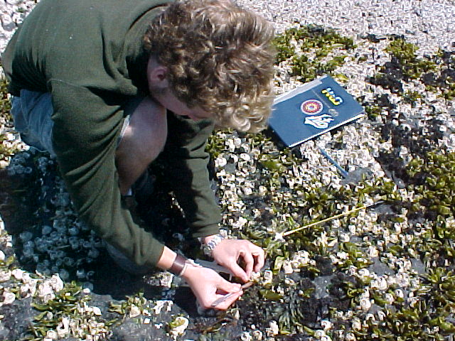
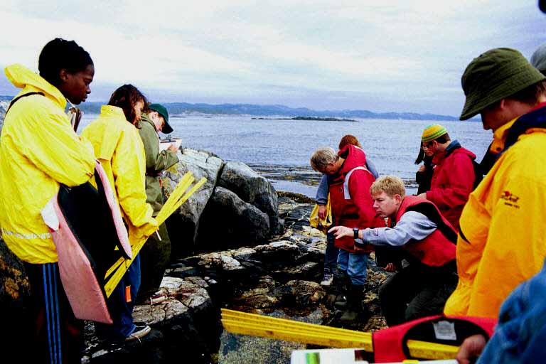
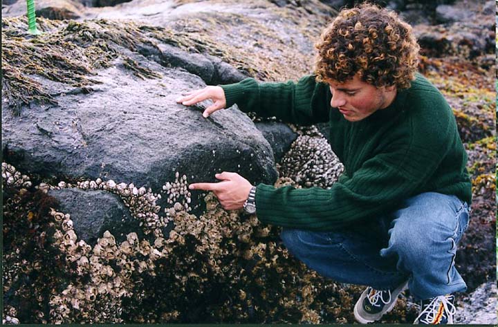
The author working with Halosaccion glandiforme at Race Rocks Ecological Reserve.
The Experimental and Control Groups Used
In using three transect belts the correlation between variables is based on a wider average of results. By setting all three transects to begin at the zero meter tide level they can be accurately compared. In taking the transect belts in proximity to one another they are more likely to be of similar conditions. For example, all three transects were on the same side of Race Rocks facing the same swell and wind directions. Therefore more variables are eliminated that could make comparison amongst them more obscure.
Instruments used
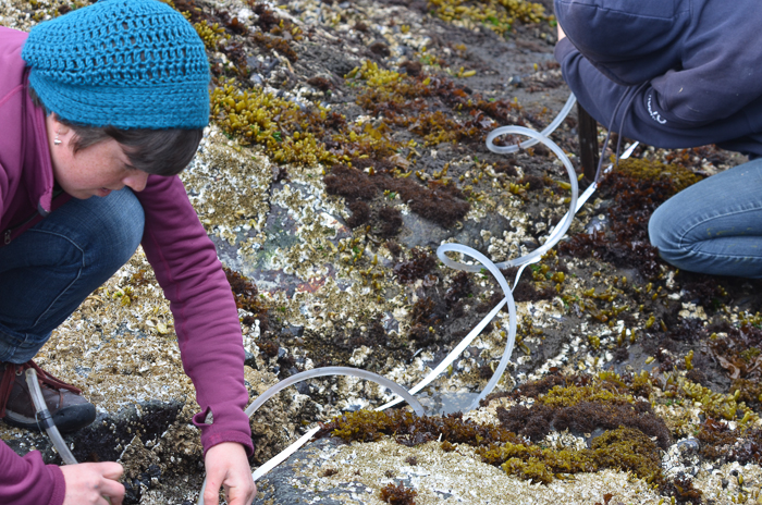
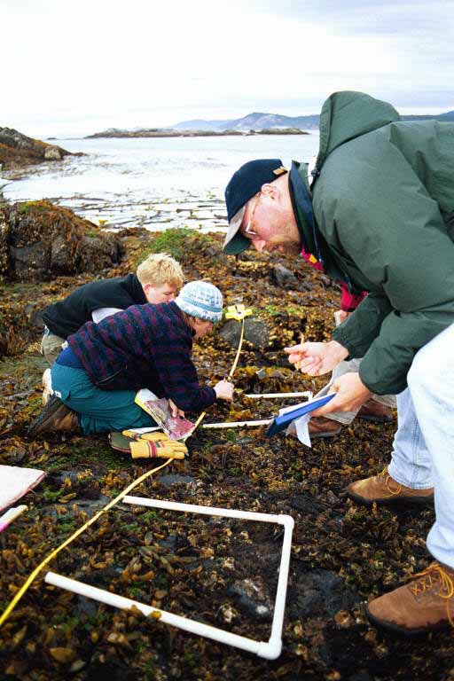
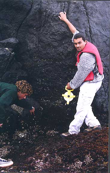
In creating the belt transects, a measuring tape over 10 meters long with markers for every meter was placed along the tidal zone tight to the rocks. The photos were taken along the measuring tape with a Sony Digital Camera. The photos were taken from about 1 meter above the ground (approximately waist height). One photo would cover a section of about fifty centimeters. The photos were taken overlapping the previous so that they could be fit together appropriately at a later time.
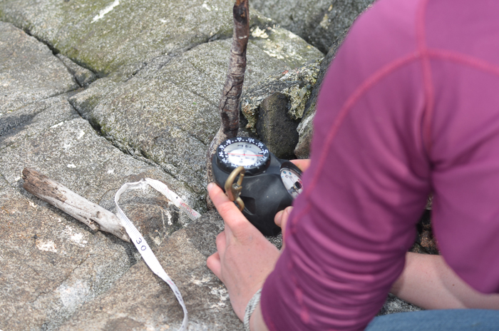
With the measuring tape in place the next step was to measure the physical height of the rock slope along the transect line. Height was measured at every 50 cm interval. A meter stick would be held perpendicular to (for example) the 1 meter mark and the 1.5 meter mark. By placing a third meter stick with a liquid level attached perpendicular to the initial stick and butting up horizontally to the second stick the difference in height was obtained.
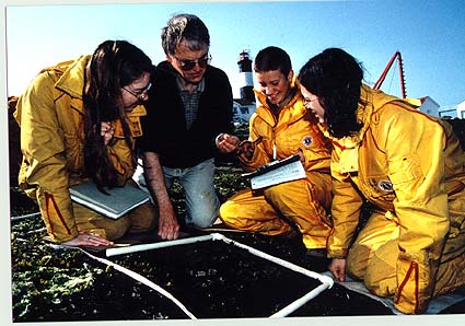
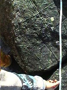
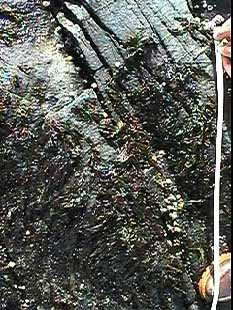
These values were recorded in a chart and then used in the making of a height and slope outline graph of the rock surface at the transect belts. In collating the individual transect photos into one cohesive transect belt the computer imaging program Adobe Photo 4 was used. After splicing the pictures appropriately the meter marks were marked by a line and each cluster of Halosaccion glandiforme was outlined for further analysis (figure 5).
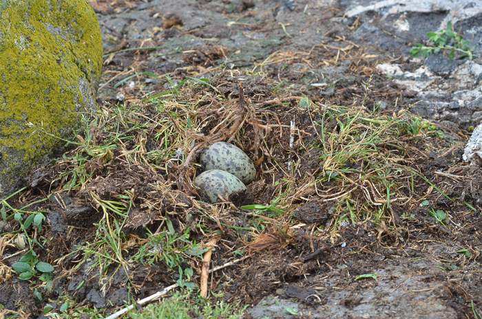
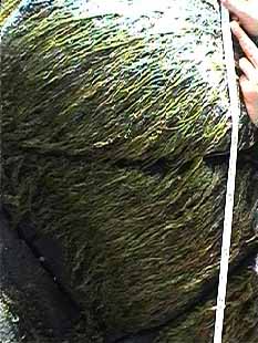
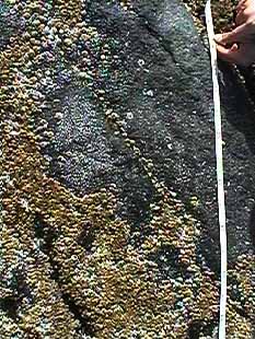
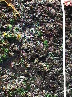
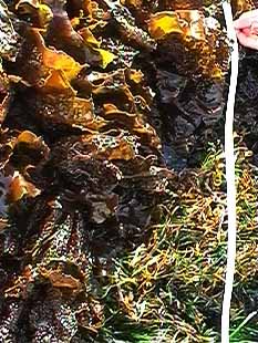
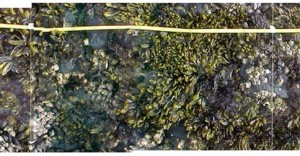 Figure 5. This image represents an example of a meter segment from the belt transect (taken from peg 6 at meter 4). The measuring tape is visible as yellow line at the top of the image. The meter segments can be seen marked by white vertical lines at the sides of the image.
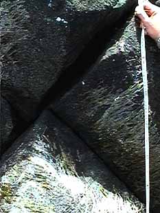
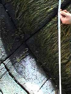
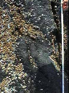
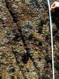
Further computer analysis was carried out using Scion Image for Windows. This program provided the capability of measuring the population density of Halosaccion glandiforme along the transect belt. The area of each transect section was measured scaled to the according meter segment length. Each meter section on the belt transect varied slightly from the others, as did the area of each meter segment. This is because of discrepancies in the distance between the camera and the shore, a source of error that is hard to avoid completely with such rough rocky intertidal terrain. Finally the total area covered by Halosaccion glandiforme clusters, as seen outlined in orange (figure 6), was measured in each meter segment. When compared to the corresponding area measurements of their meter segment the population density of Halosaccion glandiforme could be determined as a percentage covering of that area.
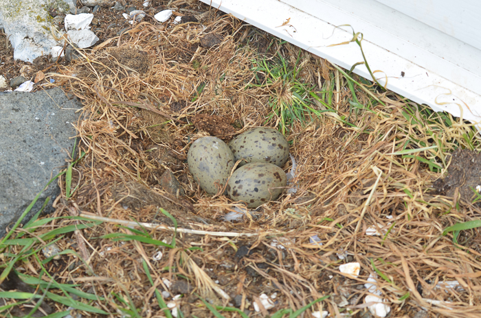
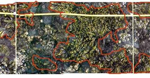
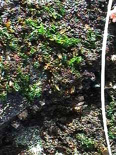
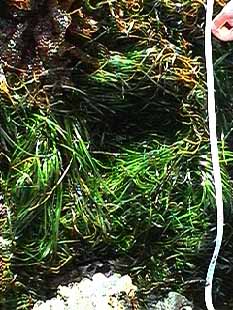
 Figure 6. This image is an example of a meter segment from a belt transect (peg6, meter segment 4). The orange outlines represent the area covered by Halosaccion glandiforme. With measurements scaled to the according meter as presented by the measuring tape the area of the meter segment and the Halosaccion coverage was calculated and compared.(For complete belt transect of peg 6 see appendix.)
Analysis of Data
Introduction
With the data obtained from the belt transects of the intertidal zone the results of height and population density were compiled into tables and subsequently graphs to represent the possible relation. Also the data for the effect of surface slope on population density was converted into a graph.
-

-
Peg 5a Click to get a very long image.
-

-
Peg 5b
-

-
Peg 6
Findings that relate to Hypothesis 1 and 2
| Transect meter segment |
Mean of height |
Percent coverage of area |
| 1 |
0 |
0 |
| 2 |
35 |
0 |
| 3 |
60 |
0 |
| 4 |
85 |
3.4 |
| 5 |
115 |
60.9 |
| 6 |
145 |
89.6 |
| 7 |
170 |
1 |
| 8 |
165 |
14.1 |
| 9 |
200 |
0 |
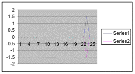
Table 1. Population density (in percent coverage of each meter segment) is shown in relation to the mean of vertical height of the corresponding meter segment from measurements at peg 5.
| Transect meter segment |
Mean of Height |
Percent coverage of area |
| 1 |
5 |
0 |
| 2 |
17 |
0 |
| 3 |
21 |
0 |
| 4 |
70 |
1.6 |
| 5 |
110 |
23.8 |
| 6 |
160 |
46.8 |
| 7 |
190 |
10.7 |
| 8 |
230 |
0 |
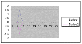
Table 2. Population density (in percent coverage of each meter segment) is listed in relation to the mean of vertical height of the corresponding meter segment from measurements at peg 5b1.
| Transect meter segment |
Mean of height |
Percent coverage |
| 1 |
2 |
0 |
| 2 |
50 |
0 |
| 3 |
132 |
26.6 |
| 4 |
170 |
49.5 |
| 5 |
190 |
0 |
| 6 |
203 |
7.1 |
| 7 |
210 |
1.4 |
| 8 |
230 |
0 |
| 9 |
258 |
0 |
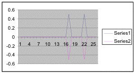
Table 3. Population density (in percent coverage from each meter segment) is shown in relation to the mean of vertical height of the corresponding meter segment from measurements at peg 6.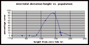
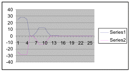
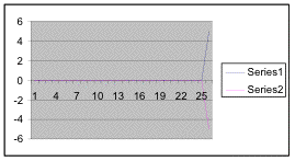
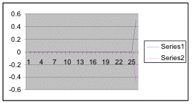
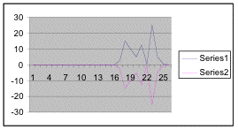
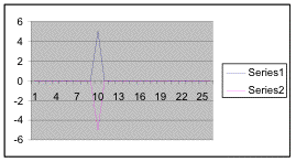
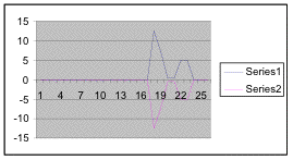
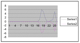
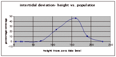
Figure 7. Graph of data from table one, peg 5. This figure represents the relation between population density (in percent coverage from each meter segment) and vertical height.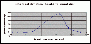
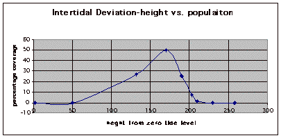
Figure 8. Graph of data from table 2, peg 5b1. This figure represents the relation between population density (in percent coverage from each meter segment) and vertical height.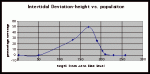
Figure 9. Graph of data from table 3, peg 6. This figure represents the relation between population density (in percent coverage from each meter segment) and vertical height.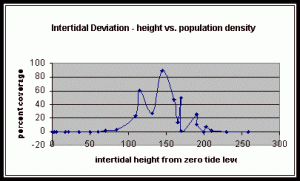
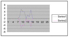
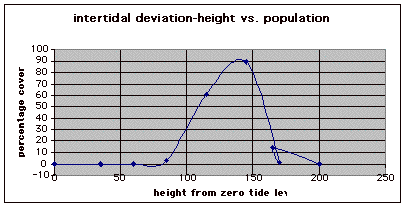
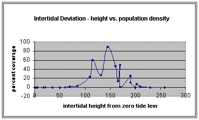
Figure 10. Graph of population density in relation to mean of intertidal vertical height with the three belt transects combined.
Statistical Analysis
| Vertical height |
Percent coverage |
| 70 |
1.6 |
| 85 |
3.4 |
| 110 |
23.8 |
| 115 |
60.9 |
| 132 |
26.6 |
| 145 |
89.6 |
| 160 |
46.8 |
| 165 |
14.1 |
| 170 |
49.5 |
| 170 |
1 |
| 190 |
25.4 |
| 190 |
10.7 |
| 200 |
0 |
| 203 |
7.1 |
| 210 |
1.4 |
From the compiled data the significant values, those values that fell within the extremes of the range of population occurrence (table 4), were used for further analysis by means of normal distribution calculations. To test the obtained values against the values expected of a normal distribution curve a graph (figure 11) was produced. Of the fifteen obtained values for vertical height the mean is 154.33 meters. Therefore the standard deviation is 43.71 meters from the mean. In accordance with a normal distribution the first standard deviation (from the mean to 110.62 and 198.04 cm) is expected to hold 34% of the values. At the second standard deviation (at 110.62 cm and 241.75 cm) 13.6% of the values are expected to be present. Finally the third standard deviation (at 23.2 cm and 285.46 cm) is expected to contain 2% of the values. With 15 values in this data set (table 4) the expected number of values for each deviation can be calculated from the expected percent (table 5).
| Expected percent |
2% |
13.6% |
34% |
34% |
13.6% |
2% |
| Expected |
0.3 |
2.04 |
5.1 |
5.1 |
2.04 |
0.3 |
| Observed |
0 |
3 |
3 |
6 |
3 |
0 |
Table 5. Data table of expected normal distribution values and obtained distribution values used in conjunction to perform chi-squared test.
The chi-squared statistic was calculated from this table (table 5) as 2.864. When this number is checked with the chi-square distribution table at five degrees of freedom it falls bellow the critical 95 percent value of 11.1. Therefore, there is a 95 percent certainty that the results fit the expectations and that the obtained values represent a normal distribution.
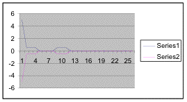
Findings that relate to hypotheses 3 and 4
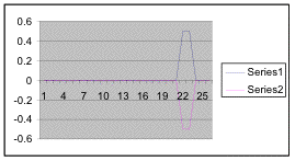
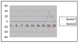
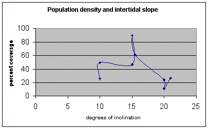
To obtain the angle of inclination for the terrain of the belt transects it was necessary to create three graphs (figures 12, 13, and 14) from the height measurements (see Instruments used) taken along the three transect lines. With the use of a protractor the angles were extrapolated from each graph (table 6). The angle measurements represent the mean of inclination for each meter segment from each transect. The calculated angles were compared to the percent coverage values that they represented. The angles are only calculated from the meter segments where a significant population density of Halosaccion glandiforme is present as slope will only be influential in the identified zone where H. glandiforme usually grows. Therefore it is mainly from the 100cm to 200cm vertical height sections of each transect belt that angle of inclination is measured.
Figure 11 (To be scanned and added later)
Figure 12 (To be scanned and added later)
Figure 13 (To be scanned and added later)
Figure 14 (To be scanned and added later)
| Angle of inclination |
Percent coverage |
| 10 |
25.4 |
| 10 |
49.5 |
| 15 |
46.8 |
| 15 |
89.6 |
| 15.5 |
60.9 |
| 20 |
23.8 |
| 20 |
10.7 |
| 21 |
26.6 |
Table 6. This data shows percent coverage in relation to the slope of the intertidal zone. Slope is measured to represent the mean slope of each meter transect segment. Slope is only taken from the segments of the three transects where there is significant population density of Halosaccion glandiforme. Therefore it is mainly from the 100cm to 200cm vertical height sections of each transect belt.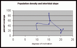
Figure 15. Graph of table 6, the relation between population density and intertidal slope.
Conclusions and Recommendations for Further Study
Interpretation and Implications of the Findings
The three individual transect graphs (Figures 7, 8, and 9) show a trend between the relationship of vertical intertidal height and the population density of Halosaccion glandiforme. The majority of Halosaccion glandiforme were found to grow between vertical heights of 100 cm and 200cm from the zero tide level. The highest recorded level of population density in each belt transect varied slightly, ranging from 145 cm vertically to 160 cm vertically. When the distribution of obtained values for height and percent coverage were compared to the normal distribution it was found that the observed results fit with 95% confidence of the expected. This suggests that the observed results are not distributed by chance occurrence but are due to a trend. The null hypothesis (Ho) is disproved and the hypothesis (Ha) is accepted, as a significant relation does exist between Halosaccion glandiforme population density and the vertical elevation on the tidal zone. It is important to place this in context however as the results are based on data from a close proximity as to decrease the variability of results. It is likely that H. glandiforme populations even on the opposite side of Race Rocks, subject to different lighting, swell action, and other possible conditions, could demonstrate a different set of results. Therefore this part of the experiment could be repeated and produce similar distribution results in the same vicinity and perhaps exhibit similar trends in a wider range of locations.
The slope percent coverage relation graph needed more data taken at more specific intervals to produce significant results. Since this relation could only be studied at heights where predetermined growth was expected it limited the data to eight significant values. The graph suggests that growth is optimum on gradients of 10 to 20 degrees with the higher population densities at 15 degrees. Yet this is not reliable as it is clear from the terrain profile graphs (figures 11, 12, and 13) that there is not a great level of variance in shoreline slope at the sites of the belt transects. There was no data collected from terrain that exhibited more extreme angles. Slope most likely affects the growing conditions of Halosaccion glandiforme however it is only one several variables that together create intertidal zonation and is therefore difficult to quantify. This study was not sufficient to come to any conclusions concerning the hypothesis and the hypothesis (Ha) is not accepted.
Recommendations
While trends were observed in this study there are many conditions that must be taken into account. The data was collected at Race Rocks in July and cannot be considered relevant for the whole year. While the H. glandiforme populations are anchored to the rock and are not likely to vary extensively in position over time, the data would be of greater accuracy if it were collected and compared over an extended time. The data collection, as previously stated, is from one limited range and has not been tested or compared with intertidal zones in any other area. For further study it would be interesting to compare growth trends in different locations. Also the percent coverage values, that were vital to findings, were calculated (using Scion Image pro.) are covered by the species. For a more in depth study, population density calculations would be more accurate if they took into account the size and number of the individual organisms. One of the most limiting factors encountered in the analysis resulted from the scale of the measurements taken. For both hypotheses the results were based on data collected from intervals of one meter along the belt transects. Any discrepancy or variation that occurred in vertical height, slope, or population density inside the transect meter segment could not be taken into account. If repeated the data analysis would be far more conclusive had measurements been taken at smaller intervals of, for example, 10cm instead of 100cm. This study focused on the intertidal organism Halosaccion glandiforme and the effects of elevation and slope on its population density. There are, however, many other variables and species that affect and grow in the intertidal zone and could be considered and tested similarly to analyze and quantify the intertidal area.
References Cited
- Waaland, Robert J. 1977, “Common Seaweeds of the Pacific Coast”. J.J. Douglas Ltd. Vancouver.
- Stephenson, T. A. and Stephenson, A. 1949, “The Universal features of zonation between tide-marks on rocky coasts.” Journal of Ecology. 37, 289-305.
- Kanwisher, J. 1957, “Freezing and drying in intertidal algae.” Biological Bulletin 113: 275-285.
- Carefoot, Thomas. 1977, “Pacific Seashores A Guide to Intertidal Ecology”. J.J. Douglas Ltd. Vancouver.
- Kozloff, Eugene N. 1996, “Seashore Life of the Northern Pacific Coast”. University of Washington Press. Seattle.
| PHOTO STRIP OF BELT TRANSECT FROM PEG#5 |
PHOTO STRIP OF BELT TRANSECT FROM PEG#5b1 |
PHOTO STRIP OF BELT TRANSECT FROM PEG#6 |


 10. USING A SPREADSHEET
 See this example .Here is a sample of the mussel distribution data as it appears on this spread sheet
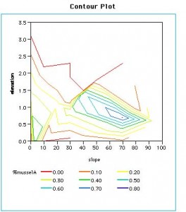 PLOTTING IN 3D


