By- Jane WatsonEd note: Our thanks to Jane Watson for taking the time to provide this possible protocol for ecological monitoring. This procedure was tried by the students but was found to be difficult to use at Race Rocks because of current, slope and exposure. It can however be adapted in part . Over 15 pegs have been established and we maintain several samples of data that are  archived in the lab at Pearson College.

What is the purpose of long-term monitoring projects?
Long-term monitoring projects are often used to follow changes in community composition or structure that occur over time. In this case you will be looking at natural changes in marine algae and invertebrate populations with respect to both long and short-term changes in water temperature.

How will this project be carried out?
You will be helping to establish the study sites which ultimately Pearson college will monitor two to three times a year. At least four of these sites will be at Race Rocks, others will be established at other sites that Pearson College divers visit regularly.

What will this involve?
Over the next three months we will be putting the permanently marked transects in. Once we have established all of the transects we will start to sample them. On each permanently marked transect Coast-watch divers will use randomly placed quadrats to estimate the abundance of selected invertebrates and algae.
In the lab the data will be entered and analyzed. These data should show how the abundance of many of many marine plants and animals change over time.
We will also be installing an underwater thermograph. This small instrument will record water temperature at predetermined intervals. Several times a year Pearson college divers will retrieve the instrument and down-load the data onto a computer. Changes in the composition of the marine community can then be examined with respect to mean temperatures, extreme temperatures and so on.
In addition to counting the abundance of marine invertebrates and algae, we will be tagging abalone, in an attempt to follow growth and mortality of individual abalone. We will also be measuring urchins which will allow us to follow changes in the population structure over time.

What will you need to know to sample these sites?
There are a number of plant and invertebrate species that you will need to be able to identify before we can sample the sites. You will also need to know how to sample using a quadrat, tag abalone and use vernier callipers… not exactly difficult stuff.
You will also need to know how to enter and analyze the data you collect. We will set things up so that this is straightforward. At the end of the school term you will be able to plot the mean abundance of the organisms we sample at all of our permanent transects. In subsequent years other Pearson College divers will continue to sample these sites.

Some species you will need to know
Invertebrates
Phylum Echinodermata

Red urchin – Strongylocentrotus franciscanus
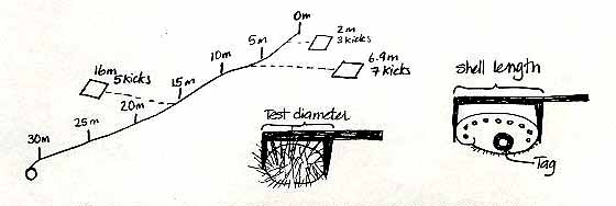
This is the most abundant of the urchins, it is unmistakable, being big and red. We will count the number of red urchins in each quadrat, as well as measuring the test diameter of the urchins. This will be done with vernier callipers. By measuring the size of the urchin tests we will be able to trace the settlement of new “recruits” and follow their growth.

Green urchin – S. droebachiensis
This is the smaller green urchin that is quite common in sheltered areas. We will count green urchins, but not measure them, unless they are very abundant at any of our sites.

Purple urchin – S. purpuratus
A small purple urchin that is generally found in the very shallow subtidal, and sometimes in the intertidal. If it occurs on any of our sites we will count them only.

Green urchins – S. droebachiensis
A small green urchin that is generally found in more sheltered waters, we will probably not encounter too many green urchins.

Giant sea cucumber – Parastichopus californicus
A large browny red sea cucumber, These are generally found in sheltered areas, or in water depths of greater than 10m. They are found on both hard and soft-bottoms.

Orange sea cucumber – Cucumaria miniata
This cucumber has a browny red body and bright orange tentacles. It is found in crevices wifli its tentacles extending beyond the crevice.

Sunflower star – Pycnopodia helianthoides
The largest of the sea stars, it can be up to lm in diameter, it comes in a variety of colours, usually orangy brown. It has up to 24 legs.

Leather star – Dermasterias imbricata
The leather star has a red back with greeny makings. It derives its name from its ieather-like texture. If you smell it (no not underwater) it has a gunpowder/garlic smell.

Beach star – Pisaster ochraceus
Yellow or purple, generally intertidal, but also found subtidally at some locations .

Painted star – Orthasterias khoeleri
Orange pink and purple, a very attractive sea star that occurs subtidally on rocky bottoms.

Blood star – Henticia spp.
This bright red, star is very common on both rocky and soft-bottomed areas.

Basket star – Gorganocephalus eucnemis
This species usually occurs in deep water, but Race Rocks is unique in having this species in shallow subtidal water.

Phylum Mollusca
Abalone – Haliotois kamtschatkana
The pinto abalone occurs from the lower intertidal to depths of about 10m. We will count, measure and tag all of the abalone we encounter. When tagged abalone are re-encountered they will be re-measured to follow growth in abalone.

Red turban snail – Astraea gibbersoa
A medium-sized snail that is very common on coralline algae. It has a hard operculum, and a shell that becomes covered with coralline algae.

Gumboot chiton – Cryptochiton stelleri
‘Ite largest chiton on our coast. You cannot see the 8 shell or plates that make up the gumboot chiton’s shell, they are hidden beneath the pinky brown tissue on the dorsal surface.

Cnidaria
Plumose anenome – Metridum senile
A very abundant bright white anenome, that does particularly well in high current areas. We will count anemones as we encounter them.

There will be other invertebrates added to this list once we determine which species are representative of the areas we are sampling.
Brown Algae
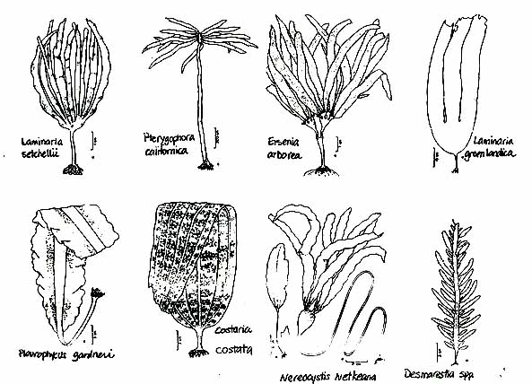Kelps – Laminariales
Bull kelp – Nereocystis luetkeana

Bull kelp is an annual species, it grows rapidly in areas that are highly disturbed. Bull kelp forms a floating canopy, it is very common at Race Rocks.

Tree kelp – Ptrerygophora californica
Tree kelp looks very much like a tree. It is a perennial species that lives in excess of 17 years. Pterygophora can be aged by cutting it down and counting the rings in its stalk or stipe. We will be tagging tree kelp on one of the transects at Race Rocks this will allow us to look at the persistence of tree kelp

Eisenia arborea
Eisenia looks very much Pterygophora, except that it has blades which are serrated at the edges, and the blades grow in two “bunches” at the top of the plant.
Laminafia setcheIlii
Laminaria groenlandica
These two species do not have a common name. Laminaria setchellii found in similar areas to Pterygophora, except that Laminaria setchellii is generally found in slightly more exposed areas.
Laminaria groenlandica is found in more sheltered areas. It looks quite different than Laminaria setchellii, since the two species are found in different areas you should have no trouble sorting them out.

Costaria costata
Costaria is really distinctive, it has three ribs on one side and two ribs on the other. It is generally an annual species but frequently manages to overwinter.

Acid weed – Desmarestia spp.
Acid weed is an annual species, which has a very “weedy” life history, it grows in highly disturbed areas, and is one of the first species to grow in areas that have been disturbed. It is very hard to count, because it forms a blanket over the sea floor, to count it you have to go down to the holdfast.

Pleurophycus gardneri
This species is generally found in very shallow areas in wave-washed areas. It is very distinctive.

There will be other species of algae that we add to our list.

 

 

---

SAMPLING
To sample the invertebrates at each of the permanently marked sites we will be using quadrats. Most of you will have done quadrat sampling before.
We will be using a random – sampling method, in which quadrats are placed randomly along / or near the transect line, and the selected invertebrates and algae in each quadrat will be counted. From these data we will calculate the mean (average) abundance as well as the variation in abundance that occurs at each site. These data will plotted in graphs which compare the abundance of each species over time, and with respect to changes in temperature.
We will go over the sampling methods prior to starting the project. All data will be recorded on data sheets pre-printed on underwater paper. An example of the type of data sheet we will be using is attached.

RACE ROCKS SAMPLING PROGRAMMELong-term sampling, a review

Long-term sampling programmes are often used to follow changes in the abundance of plants and animals over time. We will be looking at changes in the abundance of algae and invertebrates at Race Rocks. These changes will be examined with respect to changes in water temperature. The sampling method we will be using is called a stratified-random sample.

What is stratified random sampling?

In a stratified random sample we will sample the sea floor in a random manner, that is there will be no predetermined pattern to the sampling programme. The samples will be stratified because we will make sure that three depths are represented equally in our random samples.

What will we need?
Each dive pair will need
– a 30m tape measure
– a 0.7m X 0.7m quadrat (0.5m squared)
– a clip board and data sheet (with pencil)
– a slate (with pencil)
– a pair of vernier calipers
– pre-mixed epoxy, and petersen discs
– a set of 20 random number

How will we sample?
We have established 6 permanent transects around Race Rocks. Each transect is 30 metres long and runs from the shallow subtidal to about 10m depth. Once a dive pair has located the transect they will be working on, a tape measure will be tied to the shallowest pin (the 0 metre pin) and laid out down to the last pin (30 metre pin).

Before the dive, each dive pair will determine a set of 20 random numbers from a random number table (attached to these pages). There will be two numbers, both between 0 and 9. The first number will refer to the distance along the tape measure, let us say 6.9 metres (it will be the first two numbers, where-ever you start on the table, ie:69). The second number, let us say 7, will refer to the number of flipper kicks right or left of the line. The dive pair will swim along the tape locate the 6.9 mark, then left 7 kicks to the right or left of the 6.9 metre mark. After 7 kicks the diver drops the quadrat and starts to count all the invertebrates and seaweed in the quadrat.

While one diver does the counting and recording, the second diver will measure all of the sea urchins in the quadrat, recording the test diameter of each sea urchin to the nearest cm. Likewise the length of any abalone in the quadrat should also be measured, the abalone should also be tagged, using epoxy and a Petersen disc tag. The tag number should be recorded along with the length of the ablaone. Any abalone you see outside of the quadrat can also be measured and tagged.

Once the quadrat count and the measuring is completed, the dive pair returns to the tape measure, and repeats the process, using the next set of random numbers. In total divers will sample 20 quadrats between 0-10m (10 quadrats on the right side of the line, 10 quadrats on the left side), 20 quadrats between 10-20m and 20 quadrats between the 20-30m, for a total of 60 quadrats per transect. The transects will be sampled twice a year.

 Once the dive pair has sampled 20 quadrats from between the 0-10 pins, they move down to the 10-20 metre pins and repeat the process, as time and air supply allow. If it is easier, three dive pairs can work on each transect line, one dive pair working in the 0-10m area, the next pair in the 10-20m area and the third pair in the 20-30m area. Dividing the transect into three areas is the stratified part of the sampling design, using the random number table is the random part of the sampling design.

Back at the College

Wash all the sampling gear you used with fresh water, and return to its appropriate place. Back in the lab you will need to wash the salt off your data sheet, and copy the sea urchin measurements and abalone tag/measurements onto the back of the data sheet for the section of the transect line you and your partner sampled. You will also need to make sure that all of your numbers are readable, and that you have filled in all of the blanks on the data sheet.

During later lab periods you will be entering this data, and calculating the average (mean) density of the animals and seaweed you counted along each transect line. Subsequent years of Pearson College students will continue this sampling programme to generate a long-term view of how invertebrate and algae abundance changes over time.

Following is a page of random numbers, you should make sure that you are comfortable using this table. Likewise there is a data sheet, please make sure that you are familiar with the species listed on the data sheet, and that you will be able to identify them underwater.

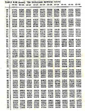
Random number table — 10,000 random numbers

27791 82504 33523

33147 46058 92388

67243 10545 40269

78176 70368 95523

70199 70547 94331

The first ten numbers in the last line are interpreted as: 7.0 m 1 kick, 9.9 m 7 kicks, 0.5 m 4 kicks, 7.9 m 4 kicks

TABLE B.39 (cont.) TEN THOUSAND RANDOM DIGITS

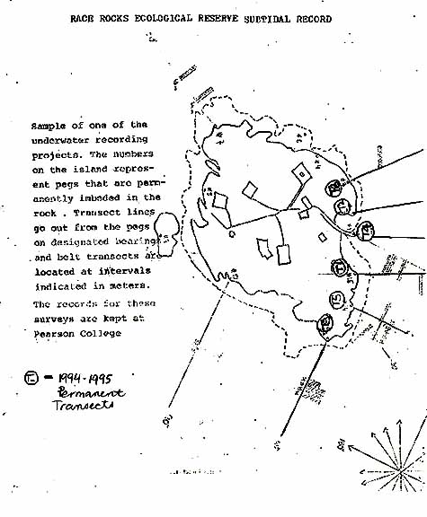RACE ROCKS ECOLOGICAL RESERVE SUBTIDAL RECORDSample of one of the underwater recording projects. The numbers on the island represent pegs that are permanently imbedded in the rock. Transect lines go out from the pegs on designated bearings and belt transects are located at intervals indicated in meters. The records for these surveys are kept at Pearson College.

T = 1994-1995 permanent transects

 

There will be other species of algae that we add to our list.

 

 

 

Sampling

To sample the invertebrates at each of the permanently marked sites we will be using quadrats. Most of you will have done quadrat sampling before.

We will be using a random – sampling method, in which quadrats are placed randomly along / or near the transect line, and the selected invertebrates and algae in each quadrat will be counted. From these data we will calculate the mean (average) abundance as well as the variation in abundance that occurs at each site. These data will plotted in graphs which compare the abundance of each species over time, and with respect to changes in temperature.

We will go over the sampling methods prior to starting the project. Data will be recorded on data sheets pre-printed on underwater paper.

RACE ROCKS SAMPLING PROGRAMMELong-term sampling, a review

Long-term sampling programmes are often used to follow changes in the abundance of plants and animals over time. We will be looking at changes in the abundance of algae and invertebrates at Race Rocks. These changes will be examined with respect to changes in water temperature. The sampling method we will be using is called a stratified-random sample.

What is stratified random sampling?

In a stratified random sample we will sample the sea floor in a random manner, that is there will be no predetermined pattern to the sampling programme. The samples will be stratified because we will make sure that three depths are represented equally in our random samples.

What will we need?

Each dive pair will need

– a 30m tape measure

– a 0.7m X 0.7m quadrat (0.5m squared)

– a clip board and data sheet (with pencil)

– a slate (with pencil)

– a pair of vernier calipers

– pre-mixed epoxy, and petersen discs

– a set of 20 random number

How will we sample?

We have established 6 permanent transects around Race Rocks. Each transect is 30 metres long and runs from the shallow subtidal to about 10m depth. Once a dive pair has located the transect they will be working on, a tape measure will be tied to the shallowest pin (the 0 metre pin) and laid out down to the last pin (30 metre pin).

Before the dive, each dive pair will determine a set of 20 random numbers from a random number table (attached to these pages). There will be two numbers, both between 0 and 9. The first number will refer to the distance along the tape measure, let us say 6.9 metres (it will be the first two numbers, where-ever you start on the table, ie:69). The second number, let us say 7, will refer to the number of flipper kicks right or left of the line. The dive pair will swim along the tape locate the 6.9 mark, then left 7 kicks to the right or left of the 6.9 metre mark. After 7 kicks the diver drops the quadrat and starts to count all the invertebrates and seaweed in the quadrat.

While one diver does the counting and recording, the second diver will measure all of the sea urchins in the quadrat, recording the test diameter of each sea urchin to the nearest cm. Likewise the length of any abalone in the quadrat should also be measured, the abalone should also be tagged, using epoxy and a Petersen disc tag. The tag number should be recorded along with the length of the ablaone. Any abalone you see outside of the quadrat can also be measured and tagged.

Once the quadrat count and the measuring is completed, the dive pair returns to the tape measure, and repeats the process, using the next set of random numbers. In total divers will sample 20 quadrats between 0-10m (10 quadrats on the right side of the line, 10 quadrats on the left side), 20 quadrats between 10-20m and 20 quadrats between the 20-30m, for a total of 60 quadrats per transect. The transects will be sampled twice a year.

Once the dive pair has sampled 20 quadrats from between the 0-10 pins, they move down to the 10-20 metre pins and repeat the process, as time and air supply allow. If it is easier, three dive pairs can work on each transect line, one dive pair working in the 0-10m area, the next pair in the 10-20m area and the third pair in the 20-30m area. Dividing the transect into three areas is the stratified part of the sampling design, using the random number table is the random part of the sampling design.

Back at the College

Wash all the sampling gear you used with fresh water, and return to its appropriate place. Back in the lab you will need to wash the salt off your data sheet, and copy the sea urchin measurements and abalone tag/measurements onto the back of the data sheet for the section of the transect line you and your partner sampled. You will also need to make sure that all of your numbers are readable, and that you have filled in all of the blanks on the data sheet.

During later lab periods you will be entering this data, and calculating the average (mean) density of the animals and seaweed you counted along each transect line. Subsequent years of Pearson College students will continue this sampling programme to generate a long-term view of how invertebrate and algae abundance changes over time.

Insert Random number table and data sheet.

Following is a page of random numbers, you should make sure that you are comfortable using this table. Likewise there is a data sheet, please make sure that you are familiar with the species listed on the data sheet, and that you will be able to identify them underwater.

Random number table — 10,000 random numbers

27791 82504 33523

33147 46058 92388

67243 10545 40269

78176 70368 95523

70199 70547 94331

 

 

The first ten numbers in the last line are interpreted as: 7.0 m 1 kick, 9.9 m 7 kicks, 0.5 m 4 kicks, 7.9 m 4 kicks

TABLE B.39 (cont.) TEN THOUSAND RANDOM DIGITS

RACE ROCKS ECOLOGICAL RESERVE SUBTIDAL RECORDSample of one of the underwater recording projects. The numbers on the island represent pegs that are permanently imbedded in the rock. Transect lines go out from the pegs on designated bearings and belt transects are located at intervals indicated in meters. The records for these surveys are kept at Pearson College.

T = 1994-1995 permanent transects

There will be other species of algae that we add to our list.

Sampling

To sample the invertebrates at each of the permanently marked sites we will be using quadrats. Most of you will have done quadrat sampling before.

We will be using a random – sampling method, in which quadrats are placed randomly along / or near the transect line, and the selected invertebrates and algae in each quadrat will be counted. From these data we will calculate the mean (average) abundance as well as the variation in abundance that occurs at each site. These data will plotted in graphs which compare the abundance of each species over time, and with respect to changes in temperature.

We will go over the sampling methods prior to starting the project. Data will be recorded on data sheets pre-printed on underwater paper. An example of the type of data sheet we will be using is attached.